Introduction
Graphing linear inequalities is a fundamental topic in algebra that teaches students to represent and analyze relationships between variables. These inequalities are essential for solving real-world problems, enabling us to express various possibilities rather than one exact value. This article shall tackle graphing linear inequalities, their key concepts, illustrative examples, and real-life applications.
Grade Appropriateness
Graphing linear inequalities is typically taught in Pre-algebra and Algebra I courses, usually taken by middle school students (grades 6-8) and early high school (grades 9-10).
Math Domain
The study of graphing linear inequalities falls within the broader mathematical domain of algebra.
Applicable Common Core Standards
The following Common Core Standards for Mathematics apply to the topic of graphing linear inequalities:
7.EE.B.4: Use variables to represent quantities in a real-world or mathematical problem and construct simple equations and inequalities to solve problems by reasoning about the quantities.
6.EE.B.8: Solve real-world and mathematical problems by writing and solving equations of the form x + p = q and px = q for cases in which p, q and x are all nonnegative rational numbers
8.EE.C.7: Solve linear equations in one variable.
Definition
A linear inequality is an inequality that involves linear expressions. It can be written in the form:
Ax + By < C,
Ax + By ≤ C,
Ax + By > C, or
Ax + By ≥ C,
where, x and y are variables and,
A, B, and C are constants.
Graphing linear inequalities is the process of plotting the solution set of the inequality on a coordinate plane.
Key Concepts
Linear inequality: A mathematical statement that involves linear expressions connected by inequality symbols (<, >, ≤, or ≥).
Graph: An organized visual representation of data and values using lines, shapes, and colors. Graphs may also be called charts, usually with two or more points showing the relationship between values.
Coordinate plane: A two-dimensional plane with x and y axes to represent and analyze relationships between variables.
Boundary line: The line that divides the coordinate plane into two half-planes, representing the equation obtained by replacing the inequality symbol with an equal sign.
Shading: The process of highlighting the region in the coordinate plane containing the inequality’s solution set.
Key Steps
Graph the boundary line.
Change the inequality to the equality symbol and isolate the variable y. Write the equation in slope intercept form (y=mx+b).
The boundary line that you will graph will depend on the inequality (>,≥, <, ≤ ).
A less than < or greater than (>) is a strict inequality. Therefore, you need to draw a dashed line.
A less than or equal to (≤ ) or greater than or equal to ( ≥) sign is a non-strict inequality. Therefore, you need to draw a solid line.
Select a test point, not on the boundary line.
Select a point not on the line and test its coordinates in the original inequality to determine whether to shade above or below it.
Substitute the test point for the inequality.
The region above or below the line containing the point will be shaded if the coordinates of the point satisfy the inequality.
Shade one side of the boundary line.
The solution set for the inequality is the entire shaded region.
Discussion with Illustrative Examples
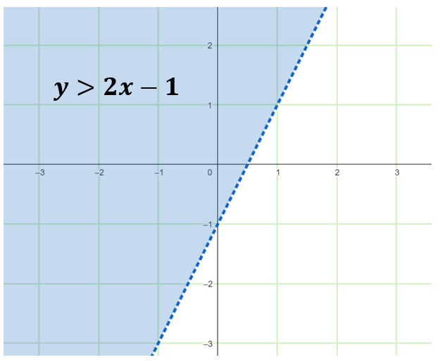
Example 1: Graph the linear inequality y> 2x – 1
Solution:
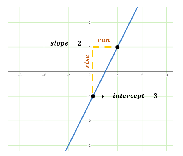
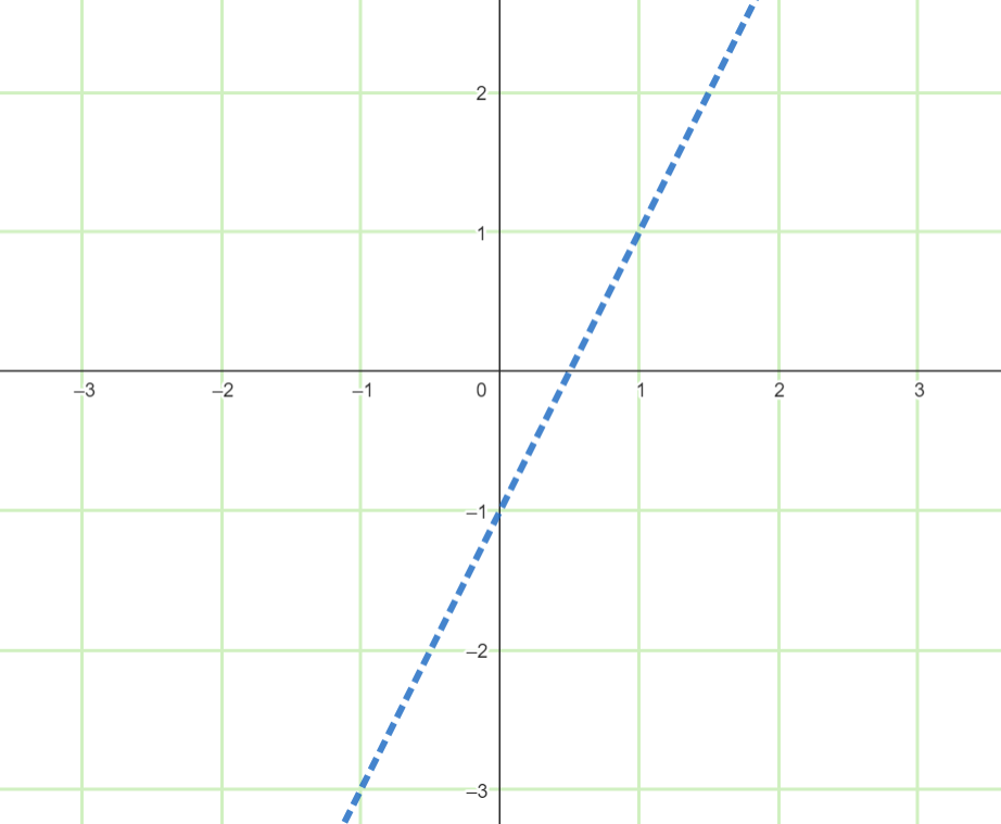
Graph the boundary line: y = 2x – 1.
Since the equation is written in the slope intercept form y=mx+b, therefore, m (slope)=2 while b (y-intercept)=-1
Since the given is a strict inequality greater than (>), then a dashed line must be used.
Select a test point not on the boundary line, like (0,0).
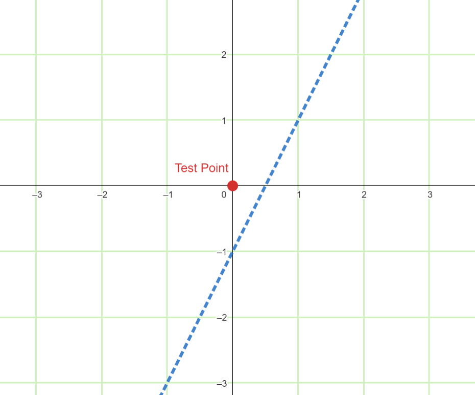
Substitute the test point into the inequality: 0 > 2(0) – 1, which is true.
Since the test point satisfies the inequality, shade the region containing the test point.
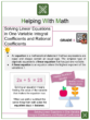
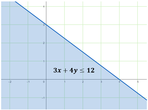
Example 2: Graph the linear inequality 3x + 4y ≤ 12
Solution:
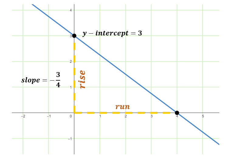
Graph the boundary line: 3x + 4y = 12.
Isolate the variable y and write the equation in the slope-intercept form (y=mx+b).
3x+4y=12
4y=-3x+12
y=-¾x+3
Select a test point not on the boundary line, like (0,0).
Substitute the test point into the inequality: 3(0) + 4(0) ≤ 12, which is true.
Shade the side of the boundary line that includes the test point since the test point satisfies the given inequality. Since the given is a non-strict inequality greater than or equal to (≤), then a solid line must be used.
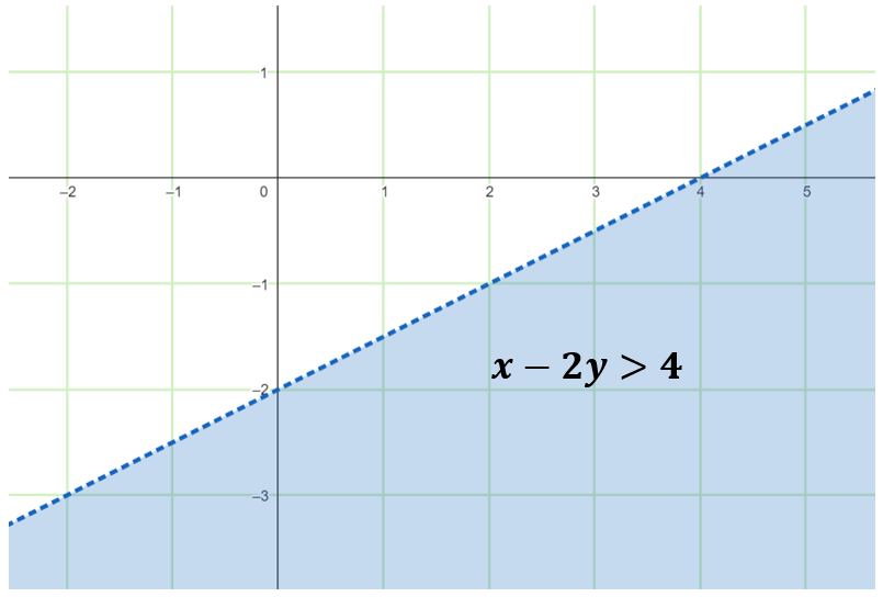
Example 3: Graph the linear inequality x – 2y > 4.
Solution:
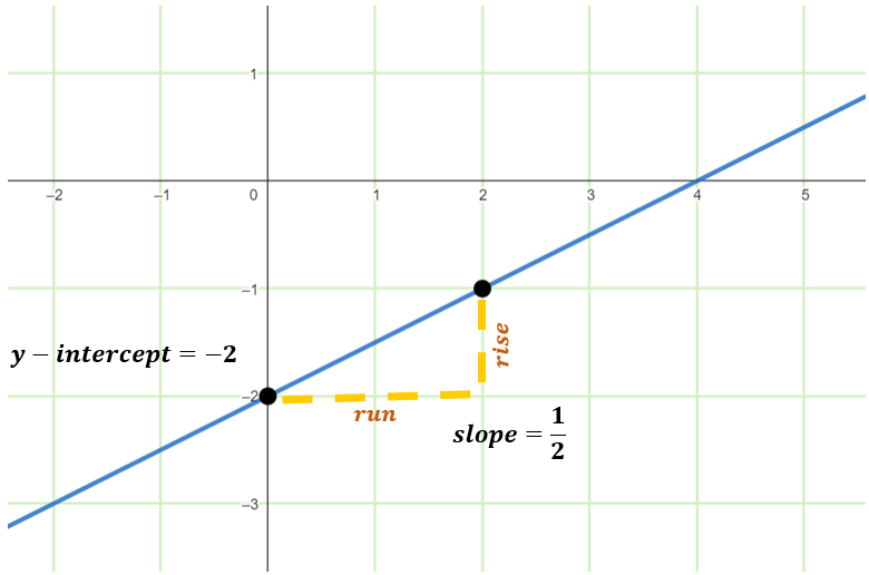
Graph the boundary line: x – 2y = 4.
Isolate the variable y and write the equation in the slope-intercept form (y=mx+b).
x-2y=4
-2y=-x+4
y=½x-2
Select a test point not on the boundary line, like (0,0).
Substitute the test point into the inequality: 0 – 2(0) > 4, which is false.
Shade the region of the boundary line that does not include the test point because the test point does not satisfy the inequality. Since the given is a strict inequality greater than (>), then a dashed line must be used.
Real-life Application with Solution
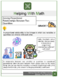
During his break, Joseph has a maximum meal budget of $9. He must pay $2 for drinks and $3 for food. How many different drinks and food combinations are available for purchase?
Solution
Let x be the number of drinks, and y be the number of food.
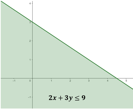
Since Joseph has a maximum meal budget of $9, we will use the inequality 2x+3y≤9.
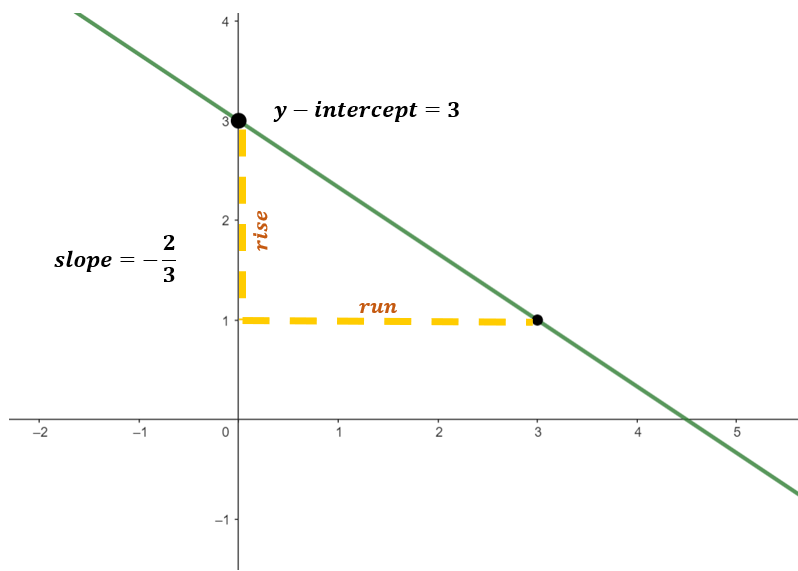
Below is the graph of 2x+3y=9, which in slope-intercept form is y=-2⁄3x+3.
Substituting the test point 0,0 into the inequality,
2x+3y ≤ 9
20+30 ≤ 9
0 ≤ 9 True
Shade the side of the boundary line that includes the test point because the test point (0,0) satisfies the inequality. Since the given is a non-strict inequality, less than or equal to (≤), then a solid line must be used.
Since we want to identify the number of possible drinks and food combinations, we must locate points in the shaded region that are positive integers.
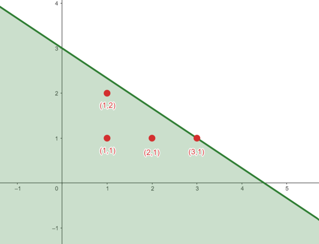
The table below shows what these points represent.
| Combinations | ||
| Number of drinks($2) | Number of food($3) | Total |
| 1 drink = $2 | 1 food = $3 | $5 |
| 1 drink = $2 | 2 food = $6 | $8 |
| 2 drinks = $4 | 1 food = $3 | $7 |
| 3 drinks = $6 | 1 food = $3 | $9 |
Notice that when we substitute the x and y values to the inequality, the total results to less than or equal to $9.
Therefore, there are four different combinations formed for drinks and food.
Practice Test
1. Graph the linear inequality y < x + 3.
2. Graph the linear inequality 2x – y ≥ 6.
3. A company produces two products, A and B. They need at least three units of A and four units of B to meet demand. If x is the number of units (A) and y represents the number of units (B), graph the inequality representing the minimum production requirements.
4. Graph the system of linear inequalities: x + y ≤ 5, x ≥ 1, y ≥ 2.
5. The sum of two numbers is less than 10, and the first is at least 3. Graph the inequality representing this situation.
Frequently Asked Questions (FAQs)
Can linear inequalities have infinitely many solutions?
Yes, the solution set for a linear inequality typically consists of infinitely many points in the coordinate plane.
How do I determine whether to use a solid or dashed line for the boundary line?
Use a solid line when the inequality includes “≤” or “≥” and a dashed line when it has “<” or “>.”
How do I graph a linear inequality with two variables?
First, graph the boundary line, the equation you get by replacing the inequality symbol with an equal sign. Then, choose a test point not on the boundary line and substitute it into the inequality. Shade the side of the boundary line that satisfies the inequality.
What is the difference between a linear equation and a linear inequality?
A linear equation is a statement that two expressions are equal, while a linear inequality is a statement that one expression is >, <, ≥, or ≤ to another expression.
How to solve a given system of linear inequalities?
In solving a system of linear inequalities, graph each inequality individually, and find the region where the shaded areas of all inequalities overlap. This overlapping region represents the solution set for the system.
Recommended Worksheets
Graphing Linear Inequalities (Civil Rights Movement Themed) Math Worksheets
Graphing and Solving Systems of Linear Equations in Two Variables 8th Grade Math Worksheets
Solving Word Problems Involving Linear Equations and Linear Inequalities 7th Grade Math Worksheets