Two variables inequality
Definition:-
When keywords other than equal to, such as greater than or less than, are used to connect two expressions with two variables, is called an inequality in two variables.
Here are some examples of two-variable linear inequalities:
Examples
- 2x<3y + 5 +1 0
- 27x^2−2y^2 < -7
- 83x^2233+4y+3≤ 6x
- 10 y−5y+x≥0
Counter examples
- X + y + z > 0
- X^2 – yz <5
- X + 6 > 0
Linear Inequalities in two variables
Two variables inequalities may be linear or non linear. When power of both variables is 1 then it is linear and more than one is called non linear, the non linear may be qualities quadratic and may be higher order.
When keywords other than equal to, such as greater than or less than, are used to connect two expressions with two variables, is called an inequality in two variables.
Here are some examples of two-variable linear inequalities:
- 2x + 3y + 5 > 0
- 2x- 3y + 5 <= 0
- 83x + 4y + 3≤ 6x
- 83x + 4y + 3 ≤ 6x
How Can We Solve Two-Variable Linear Inequalities?
Whenever the variables of x and y are swapped into a linear inequality in two variables, such as
Ax + By > C, the solution is an ordered pair (x, y) that gives a true assertion.
The distinction between solving linear inequalities and solving mathematical equation is the disparity symbol. Linear inequalities are solved in the same way that linear equations are.
Step 1: Using the laws of inequality, simplify the inequality on both sides, LHS and RHS.
Step 2: After obtaining the value, we have:
Inequalities with stringent inequalities, the two sides of the inequalities cannot be equal.
Non-strict inequalities are those in which both sides of an inequality can be equal.
Take the following disparity into account:
2x + 3y > 10
Whenever we speak about finding an answer to this inequality, we’re referring to all the pairings of x and y values that satisfy the inequality. This suggests that x = 4 , y = 2 is one of the viable solutions to this specific inequality. However, x = 0 , y = 0 isn’t since it’s less than 7 when you replace x and y equal to 0 on the LHS of the contradiction.
How can we graph two-variable inequalities?
There are infinite sets or arbitrarily many ordered pair solutions to linear inequalities in two variables.
- In the proper half of a rectangular coordinate plane, these ordered pairings or solution sets can be charted.
- In need to graph two-variable inequalities,
- Determine the form of inequity (greater than, less than, greater than or equal to, less than or equal to).
- Draw a dashed (in the event of strict inequality) or solid boundary line (in case of non-strict inequalities).
- Choose to have a test point, which is most likely (0,0) or any other non-boundary point.
- Shade the area appropriately. Shade the region that contains the test point if it solves the inequality. Color an other side of the border line if necessary.
- Check using a larger number of test points both inside and outside the region.
Important points that should be kept in mind while solving
- Inequalities can be addressed by multiplication or division both sides of the equation by the same integer.
- The direction of the inequality can be changed by dividing or multiplying either sides by negative values.
- Beyond the colored zone, ordered pairs do not solve linear inequalities.
- The terms less and larger than are strict inequalities, although less than or equal to and greater than or equal to are not.
- Every line will split the plane in which it is drawn into two halves.
- Linear inequalities’ solution sets correlate to half-planes, while linear equations’ solution sets correspond to lines.
Example
Two equations must be known in order to discover the solution of a linear equation in two variables.
Example
Consider the following scenario:
30 = 5x + 3y
The equation above involves two variables: x and y.
This equation can be depicted visually by setting the variables to zero.
When y=0, the value of x is
30 = 5x + 3(0)
x = 6
And when x = 0 the value of y is,
30 = 5 (0) + 3y
y = 10
graph of the equation is as follows
It is now clear that in order to solve a linear equation in two variables, the two equations must first be determined, after which the substitution approach can be used. Let’s look at a few examples to help you understand.
The graph of a linear inequality’s solution set is always a region. The border, on the other hand, may not necessarily be included in that set. Because of the “or equal to” element of the inclusive inequality in the preceding example, the line was included in the solution set. We would use a dashed line to indicate that all those points aren’t included in solution set when we have a rigorous inequality.
Unique solution
If and only if the specified linear equations in two variables meet at a single point, the solution will be unique for both equations.
The slope of the line created by the two equations should not be equal in order to obtain the unique solution for the supplied linear equations.
Consider these two slopes of equations of two lines in two variables, m1 and m2. If there is just one solution to the equations, then: m1 not equal to m2.
Condition for no solution
There is no solution.
If the slope values of the two linear equations are equal, the equations will have no solutions.
m1 = m2
So because lines are parallel and do not intersect, this is the case.
Example
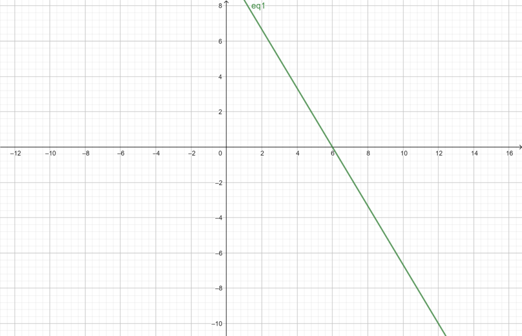
We understand that a two-variable linear equation has an infinite number of ordered pair solution that, when graphed, form a line. A linear inequality with two variables, but at the other hand, has a solution set that encompasses a half-plane region.
Y > 5x + 4
Look at shaded region as our inequality “>” used so, shaded area is away from the origin. Nut when our inequality will use < then shaded area of solution is towards origin.
Note: origin mean in graph points (0,0)
The darkened region’s boundary is defined by the line in the inequality. This means that any ordered pair in the shaded region will meet the inequality, including the border line. Choose a few test points and insert them into the inequality to determine if this is the case.
Hence,
As previously demonstrated, memorizing graphs in lower dimensions does not improve knowledge of graphs in higher dimensions. When the concepts of variability and dynamic interactions are linked with the action perspective, actions can be interiorized into processes. In this regard, alternative explanations for graphs of inequalities are needed, which can replace the existing teaching approach, the solution test. In fact, the solution test primarily promotes the action viewpoint by examining the truth value(s) for inequalities at one or more places, with no particular emphasis on variation, procedure, or empirical viewpoints.
Important Points to Remember
There are an unlimited number of ordered pair solutions for linear inequalities with two variables, which can be graphed by shading in the appropriate half of a rectangular coordinate plane.
To graph the solution set of a two-variable linear inequality, start by graphing the border with a dashed or solid line, depending on the inequality. Use a dashed line for the boundary if the inequality is strict. Use a solid line if you’re provided an inclusive inequality. After that, pick a test location that isn’t on the boundary. Shade the region that contains the test point if it satisfies the inequality; else, shade the other side.
It is a good practice to test numbers in and out of the solution set while graphing the solution sets of linear inequalities as a check.
Nonlinear Inequality Graphing
Many of the equations in the systems we’ve seen so far have been equalities, but we may come across systems with inequalities as well. We already know how to graph linear inequalities by first graphing the related equation and then shading the region denoted by the inequality symbol. To understand how to solve systems of nonlinear inequalities, we’ll use the same procedures to graph a nonlinear inequality. An inequality with a nonlinear expression is called a nonlinear inequality. A nonlinear inequality is similar to a linear inequality in terms of graphing.
Remember that the graph is presented with a dashed line when the inequality is higher than, y > a, or less than, y a. The graph is presented with a solid line when the inequality is higher than or equal to, y a, or less than or equal to, y a. The graphs will form regions in the plane, and each region will be tested for a solution. If one point in the region functions properly, the entire region functions properly.
Quadratic inequality in two variables
Definition
One of the following formulations can be used to express quadratic inequalities in two variables:
Where a, b, and c are all real numbers, and y > ax^2 + bx +c
X < y^2 +by +c
Ax^2+Bx+c – y > 0
A region of the Plane with a parabola as the border is defined by a quadratic inequality in two variables. The set of points (x, y) that are solutions to a quadratic inequality is known as the graph. The solution zone can be above or below the parabola, and the points on the parabola can be included or excluded.
How and when to Graph a Two-Variable Quadratic Inequality
To discover the roots and vertices of the curve, rewrite the inequality as a quadratic equation and solve it by completing the square.
Step 2: Draw the parabola using the roots and vertices. If y = ax2 + bx + c, the solution set for the inequality is below the curve, and if y > ax2 + bx + c, it is above the curve.
Verification is the third step. To see if the inequality holds, choose random points from both sides of the curve. If indeed the point is a solution, shade the area around it.
Example
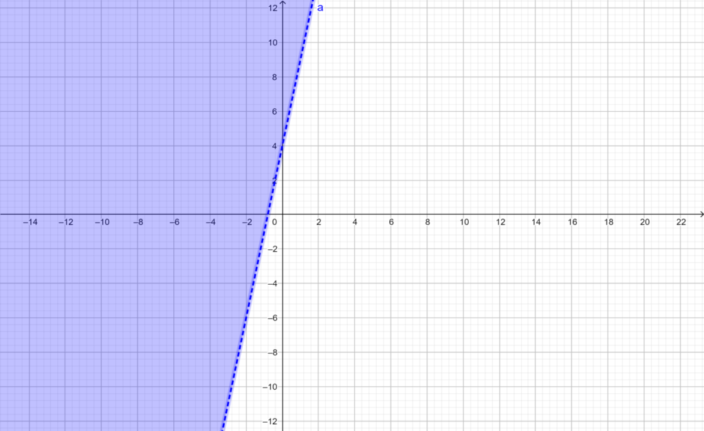
Let y > 5x^2 –x – 4
The associated equation of this inequality is as follows
0 = 5 x^2 –x – 4
Now we can either factorize this quadratic equation or apply quadratic formula and will find its roots for further processing.
Hence, by factorizing
0 = 5x^2 + 5x – 4x -4
Y0= 5x( x +1) -4( x + 1)
This implies
= (x + 1)( 5x – 4)
Hence roots are
X = -1
X = 4/5
The solution to the disparity can be found in the shaded area below.
Draw a graph for an inequality that is bounded by a parabola.
- As though it were an equation, graph the parabola. The solution set’s region is defined by this border.
- The parabola is graphed as a solid line if the border is included in the region (the operator is or).
- The parabola is graphed as a dashed line if the boundary is not included in the region (the operator is or >).
- To see if a point in one of the regions satisfies the inequality assertion, test it. The solution set is the region that includes the point if the statement is true. The solution set is indeed the region on either side of the boundary line if indeed the statement is untrue.
- The solution set is represented as a shaded region.
Alternative explanations for graphs of two-variable inequality
Preserves teachers were required to explain essential ideas contained in problems and to solve problems with extensive explanations on why they employed certain techniques or ideas in their problem solving after being taught in a classroom where relational knowledge was emphasized.
Despite having taken a class that focused on relational comprehension, 10 of the fourteen teachers failed to explain graphs of inequality at all. Two of the next four graphs were described only through the solution test, while the other two were explained using the solution test and the concept of variation. The two preserves teachers who used variation and the solution exam to explain the graphs included “near-by points” in their arguments. “A significant insight that students comprehend is that ‘near-by sites in the viable zone also meet inequalities,'” one student says.
Inequalities compounded
Compound inequalities are a group of inequalities that have either “and” or “or” in the middle. To solve inequalities in this example, simply answer each inequality separately and then determine the final solution using the principles below:
If there is a “and” between the independent inequalities, the final solution is the intersection of their solutions.
If there is a “or” between the independent inequalities, the ultimate solution is the union of their solutions.
The rules for calculating the absolute value of inequalities are the same as for calculating the absolute value of numbers. The distinction is that in the earlier, we have a variable and in the latter, we have a constant.
What is Absolute Value Inequality, and how does it affect?
Let’s review what the absolute value of a number is before learning how to solve absolute value inequalities.
The distance of a value from the origin, independent of direction, is the absolute value of a number by definition. Two vertical lines around the integer or statement denote absolute value.
The absolute value of x, for example, is represented as | x | = a, implying that x = +a and -a. Let’s look at what absolute value inequalities are.
An expression using absolute functions and inequality signs is known as an absolute value inequality. The equation |x+ y + 3| > 1 is an absolute value inequality using a greater than symbol,
The absolute value inequality contains One can choose from four distinct inequality symbols. Less than (), larger than (>), less than or equal (), and greater than or equal () are the four options. As a result, any of these four symbols can be used to represent absolute value inequalities.
Inequality of Absolute Value Graphs in Two Dimensions
If indeed the inequality is close to the equation of a line (for example, y > m|x| + b), we get a V shape with absolute value graphing, and can shade above or below the V. This is very similar to graphing two-variable inequalities. The V-shape is created by graphing inequality with absolute values.
Conclusion
- A numerical solution representing a line and a parabola can have three different sorts of solutions: (1) no solution, in which case the line does not intersect the parabola; (2) one solution, in which case the line is tangent to the parabola; and (3) two solutions, in which case the line meets the parabola in two spots.
- A system of equations representing a circle and a line can have three different sorts of solutions: (1) There is no solution because the line does not intersect the circle; (2) there is one solution since the line is tangent to the parabola; (3) there are two solutions because the line meets the circle in two points.
- There are five types of alternatives to the nonlinear system equations that reflect an ellipse as well as a circle: (1) no solution, the circle and the ellipse do not intersect; (2) one solution, the circle as well as the ellipsoid are tangent to each other; (3) two solutions, the circle and the ellipse interrelate in two points; (4) three solution provider, the circle and the ellipse intersect in three places; (5) four solutions, the circle and the
- Except for > or, we create a dashed line and shade the region containing the solution set, an inequality is graphed in the same way as an equation.
- Inequalities and equalities are handled in the same way, but systems of inequalities must fulfill both inequalities.